Cross-correlation

In this notebook we show how the CCF works and how to interpret the CCF- and Kp-V\(_{sys}\)-maps.

import numpy as np
import matplotlib.pyplot as plt
from redcross import Datacube, Planet, Template, CCF

Load reduced data

We’ll work with a reduced datacube with the main orders of HARPS-N (check out previous notebooks to learn about the reduction process).

data_dir = 'data/'
dc = Datacube().load(data_dir+'datacube_reduced_orders30-41.npy')
print('shape = {:}'.format(dc.shape))
print(dc.shape)

Loading Datacube from... data/datacube_reduced_orders30-41.npy
shape = (12, 247, 4096)
(12, 247, 4096)

Load atmospheric template

Let’s load an Fe emission template generated with petitRADTRANS (check out Notebook XX for more info on the template).

# Load template
template_path = data_dir + 'Fe_tea_template.npy'
twave, tflux = np.load(template_path)

template = Template(wlt=twave, flux=tflux).sort().convolve_instrument(res=115e3)

Cross-Correlation function

The CCF is computed for each spectrum (row of our datacube) over a range of RV-shifts as defined in the RVt vector. For each shift \(RV\) we have

\[\text{CCF} (v) = \sum_i \frac{R_i · m_i(v)}{\sigma_i^2}\]

where the sum is over wavelength channels \(i\). An efficient way to calculate the CCF is using a dot product between the weighted data \(R_i / \sigma_i^2\) and \(m_i(v)\) (see numpy.dot()).

Interpolation

The template is sampled onto the data wavelength grid and shifted for every RV value. This two steps can be performed in a single operation as shown belown

from scipy.interpolate import interp1d, splrep, splev

# Pick a wavevector from one order
wave_R = dc.order(0).wlt

# Define the RV-shift
delta_RV = 20. # km/s
c = 2.998e5 # km/s
beta = delta_RV/c
wShift = np.sqrt(((1-beta) / (1+beta)))
# Get the SHIFTED and RESAMPLED template
temp = template.copy().crop(wave_R.min(), wave_R.max()) # crop to a region around the selected order (speed up interpolation)

# 1) linear interpolation
m =  interp1d(temp.wlt*wShift, temp.flux)(wave_R)
# 2) *spline* interpolation
cs = splrep(temp.wlt*wShift, temp.flux)
m_spline = splev(wave_R, cs)

# Plot before and after
fig, ax = plt.subplots(2,1, figsize=(9,3), sharex=True, gridspec_kw={'height_ratios': [6,3]})
lw = 0.5
ax[0].plot(temp.wlt, temp.flux, lw=lw, label='Original')
ax[0].plot(wave_R, m, '--o', ms=1, lw=lw, label='Linear interp')
ax[0].plot(wave_R, m_spline, '--o', ms=1, lw=lw, label='Spline interp')

ax[1].plot(wave_R, (m_spline - m)/m_spline, '--xr', ms=1, lw=lw, label='Residuals')

ax[0].set(xlim=(4840.2, 4841.8), ylim=(0.999995, 1.000040), ylabel='Flux (1 + Fp/Fs)')
ax[0].legend()

ax[1].set( xlabel='Wavelength (A)', ylabel='Residuals \n(Spline - Linear)')

plt.show()

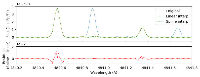
For models with resolution much higher than the data, both interpolation methods yield very similar results. Spline interpolation is faster because it is a two-step process: first it generates the B-spline decomposition of the input model once and then it projects it on the different shifted wavelength vectors (see scipy.interpolate.splrep)

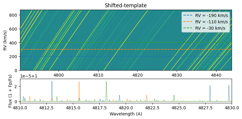
To speed up the CCF we can avoid using a loop over all RV-shifts by building a 2D-shifted-template matrix \(S_{kj}\) with shape (nShifts, nPix), hence the CCF-map is generated in one multiplication

\[\text{CCF}_{ik} = \frac{R_{ij}}{\sigma_{ij}^2} · S_{kj}^\mathrm{T}\]

where \(S_{kj}\) must be transposed so that the dot product is over the wavelength dimension.

In the next cell we generate and display the \(S_{kj}\) matrix.

# Define RV-shift vector (km/s)
RVt = np.arange(-350, 351, 0.8)

# The output is a Datacube instance
temp2D = template.shift_2D(RVt, dc.order(0).wlt)

# Display the matrix (top) and three horizontal slices (bottom) i.e. 1D-templates shifted at different RVs
fig, ax = plt.subplots(2,1, figsize=(9, 4), gridspec_kw={'height_ratios': [5,2]})
temp2D.imshow(ax=ax[0])
c = 2.998e5
for row in np.linspace(200, 400, 3, dtype=int):
    ax[1].plot(temp2D.wlt*(1+temp2D.rv[row]/c), temp2D.flux[row], lw=0.6)
    ax[0].axhline(y=row, ls='--', c=plt.gca().lines[-1].get_color(), label='RV = {:.0f} km/s'.format(temp2D.rv[row]))

ax[0].set(ylabel='RV (km/s)', title='Shifted-template')

ax[1].set(xlabel='Wavelength (A)', ylabel='Flux (1 + Fp/Fs)',
          xlim=(4810, 4830), ylim=(1. - 2*1e-6, 1+ 3*1e-5))
ax[0].legend()
plt.show()

The operations described above are performed in the function ccf.run(datacube) given an RVt vector and 1D-template template passed when creating the CCF instance.

The CCF object is an inherited class of Datacube so the same functions can be used, such as imshow() which correctly identifies the \(x\)-vector as \(RV\) instead of wavelength. The values of the CCF can be accessed with the flux attribute (e.g. ccf.flux) and the RV-vector as ccf.rv.

# merge all orders to have a datacube with shape (nFrames, nPix)
dcm = dc.merge_orders()

ccf = CCF(RVt, template).run(dcm)
# Plot the CCF-map
fig, ax = plt.subplots(1, figsize=(9, 3))

# ccf.imshow(ax=ax, fig=fig) # passing a `fig` argument will display the colorbar
ccf.imshow(ax=ax)
ax.set(xlabel='RV (km/s)', ylabel='Frame number', title='CCF-map ({:} frame)'.format(ccf.frame))
plt.show()
outfig = '/home/dario/AstronomyLeiden/MRP/report/MRP-report/plots/methods/ccf_fe.png'
fig.savefig(outfig, dpi=200, bbox_inches='tight', facecolor='white')

CCF elapsed time: 6.22 s

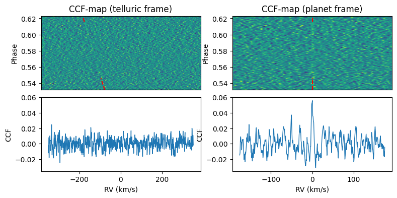
The previous map is computed in the frame of the passed Datacube (default = telluric). In the telluric (or stellar) frame, the planet trail changes in RV (as seen as a bright stripe in emission spectra). This trail becomes vertical in the planetary frame (where RV = 0).

To shift to the planetary frame we can call the function ccf.to_planet_frame(planet) to shift every frame by the expected RV of the planet (via linear interpolation). In the following cell we display the CCF-map in the planetary frame and the time-average CCF.

planet_file = 'data/wasp189.dat'
planet = Planet(file=planet_file, **dc.header)
planet.Kp = 193.5 # setting a more accurate value than the Keplerian (see Yan+2020 CO detection)

ccf_planet = ccf.to_planet_frame(planet)

• 1. The y-axis can display the phase at each frame if the attribute ccf.phase is defined.

  ccf.phase = planet.phase

• 2. To identify the planet signal in the CCF-map it can be useful to overlap the expected RV-trail. Implemented by calling

  planet.trail(ax, frame)

# Plot the CCF-map
fig, ax = plt.subplots(2,2, figsize=(9, 4))
fig.subplots_adjust(hspace=0.1)


for i,c in enumerate([ccf, ccf_planet]):
    c.phase = planet.phase
    c.imshow(ax=ax[0,i])
    ax[1,i].plot(c.rv, np.median(c.flux, axis=0), lw=1.)
    planet.trail(ax=ax[0,i], frame=c.frame)

    ax[0,i].set(xticks=[], ylabel='Phase', title='CCF-map ({:} frame)'.format(c.frame))
    ax[1,i].set(xlabel='RV (km/s)', ylabel='CCF')
ax[1,0].set_ylim(ax[1,1].get_ylim())
plt.show()