Templates

High-resolution models of emission/transmission are a key ingredient in HRCCS. When the model is ready for cross-correlation we call it a template.

In this notebook we review some of the basic steps to convert a model into a template.

To learn about how to generate such models we suggest to check out the excellent documentation of petitRADTRANS or PyratBay.

Read model

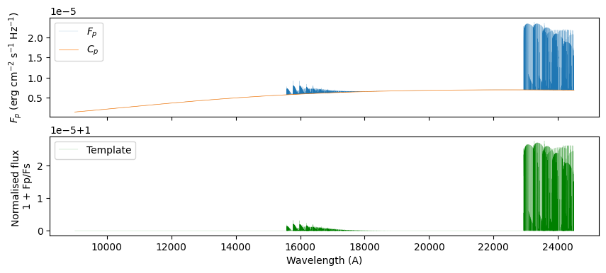
Models should contain two vectors (or three) of the same size: wavelength wave, planet flux Fp and (optionally) the planet continuum Cp.

Here we read a CO model covering the GIANO wavelength range (from 0.95 to 2.45 \(\mu\)m). This model has been generated using thermochemical-equilibrium-chemistry.

The following procedure is generic and applies to any species/TP-profile/volume-mixing-ratio for emission spectroscopy.

import numpy as np
import matplotlib.pyplot as plt
%load_ext autoreload
%autoreload 2
# constants in CGS
c = 29979245800.0 # cm/s
h = 6.62606957e-27
kB = 1.3806488e-16

def blackbody(T, nu):
    b = 2.*h*nu**3./c**2.
    b /= (np.exp(h*nu/kB/T)-1.)
    return b

The emission model \(F_p\) must be scaled to the stellar flux \(F_S\) and the transit depth \(D=\left(\frac{R_P}{R_S}\right)^2\), hence the estimated emission from the planet is

\[\text{emission} = \frac{F_{p}}{F_s}D \approx \frac{F_{p}}{B(T_{\text{eff}})}D\]

Finally, we normalise the emission model by the continuum to obtain a suitable template to cross-correlate with our data.

\[\text{continuum} \equiv C_p \approx B(T_{\text{eq}})\]

\[\text{template} = \frac{1 + \frac{F_{p}}{B(T_{\text{eff}})}D}{1 + \frac{C_p}{F_s}D}\]

Note that the continuum signal must be scaled too.

file = 'data/CO_tea_model.npy'
wave, Fp, Cp = np.load(file)

# Planet and star parameters
Rp, Rs = 1.679, 1.509
T_planet, T_star = 2273.5, 7400.
D = (Rp*0.01/Rs)**2 # transit depth

# Compute Black-Body function for the stellar continuum
freq = c/(wave*1e-8)
Fs = np.pi * blackbody(T_star, freq)

# Convert model to template
template = 1 + (D * Fp/Fs)
continuum = 1 + (D * Cp/Fs)
template /= continuum

# Plot results
fig, ax = plt.subplots(2, figsize=(10,4), sharex=True)
lw = 0.1
ax[0].plot(wave, Fp, lw=lw, label='$F_p$')
ax[0].plot(wave, Cp, lw=lw*5, label='$C_p$')

ax[1].plot(wave, template, lw=lw, c='g', label='Template')

ax[0].set(ylabel=r'$F_p$ (erg cm$^{-2}$ s$^{-1}$ Hz$^{-1}$)')
ax[1].set(xlabel='Wavelength (A)', ylabel='Normalised flux \n1 + Fp/Fs')
[ax[i].legend() for i in range(2)]
plt.show()

The above code to scale and normalise the model is equivalent to the function template.scale_model(T_star, transit_depth)

from redcross import Template

template = Template(file=file)
template.scale_model(T_star, D)

<redcross.template.Template at 0x7f073766de80>

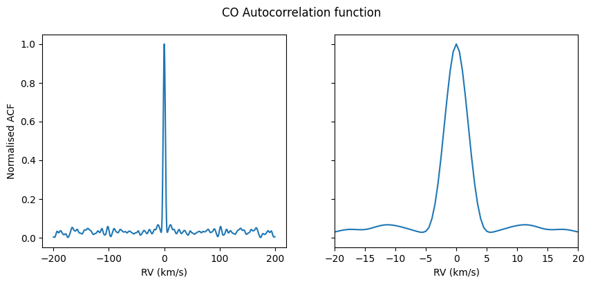
Autocorrelation function

To understand what the outcome of cross-correlating our data with a template might look like, we might want to investigate the shape of the auto-correlation function (ACF).

To speed things up, we’ll first crop the template to the region with strong CO emission lines (the right edge).

template.crop(22e3, 25e3) # arguments = (wavelength_min, wavelength_max) in same units as defined above

<redcross.template.Template at 0x7f073766de80>

from redcross import CCF
# define RV-shift vector
RVs = np.arange(-200., 200.,0.5)

# Create CCF instance and call `autoccf`
ccf = CCF(RVs, template).autoccf()

Plot the results, zooming-in around RV = 0 km/s on the right subplot

fig, ax = plt.subplots(1, 2, figsize=(10,4), sharey=True)

for i in range(2):
    f  = ccf.flux - ccf.flux.min()
    ax[i].plot(ccf.rv, f / f.max())
    ax[i].set(xlabel='RV (km/s)')
ax[1].set(xlim=(-20, 20.))
ax[0].set(ylabel='Normalised ACF')
fig.suptitle('CO Autocorrelation function')

plt.show()