Quickstart
Preparing a spectral datacube object
Let’s initialise a datacube instance that will store the wavelength and flux.
[3]:
import numpy as np
import matplotlib.pyplot as plt
from astropy.io import fits
from redcross import Datacube, CCF, KpV, Planet, Template
Load data
We load an example file containing a set of HARPS-N frames and 9 of the central orders (33 to 41).
To follow the example: download the FITS file from link and place it in data_dir. Or load your own data containing a wavelength vector (nOrders, nPixels) and a flux vector with shape (nOrders, nFrames, nPixels).
[4]:
data_dir = 'data/'
file = data_dir + 'example_harpsn33_42.fits'

with fits.open(file) as hdul:
    wave = hdul[1].data
    flux = hdul[2].data
    header = hdul[3].data # this will be used in the Cross-Correlation section
print('--Shape-- \n Wave = {:} \n Flux = {:}\n--------'.format(wave.shape, flux.shape))
print('{:} orders, {:} files, {:} pixel channels\n'.format(*flux.shape))
dc = Datacube(wlt=wave, flux=flux)
--Shape--
 Wave = (9, 4096)
 Flux = (9, 247, 4096)
--------
9 orders, 247 files, 4096 pixel channels
Display all orders
For each order, plot the master spectrum. Order 0 corresponds to order 33/69 of HARPS-N.
[5]:
fig, ax = plt.subplots(1, figsize=(14,4))
for o in range(dc.nOrders):
    dco = dc.order(o).plot(ax=ax) # .plot() displays the time-average i.e. master-spectrum

ax.set(xlabel='Wavelength (A)', ylabel='Flux (counts)')
plt.show()

Basic reduction
To manipulate the data, we will work with each order separately. To select an order simply call the function datacube.order(). Most functions accept an ax parameter to plot the resulting single-order datacube.
[6]:
dco = dc.order(0)

fig, ax = plt.subplots(4, figsize=(12, 4))
dco.imshow(ax=ax[0])
dco.normalise(ax=ax[1]) # divide each frame by its mean value
dco.sysrem(5, ax=ax[2]) # run `n` iterations of the SysRem algorithm
dco.high_pass_gaussian(window=15, ax=ax[3]) # remove low-freq signal

[ax[i].set_xticks([]) for i in range(len(ax)-1)]
ax[0].set(ylabel='Frame number')
ax[len(ax)-1].set(xlabel='Wavelength (A)')
plt.show()

Now let’s loop over all orders, the steps applied above can be concatenated in a single line
[7]:
nOrders = dc.shape[0]
for order in range(nOrders):
    print('Order {:}/{:}'.format(o, nOrders-1), end='\r')
    dco = dc.order(order) # select order
    dco.normalise().sysrem(5).high_pass_gaussian(15.) # apply reduction routine
    dc.update(dco, order) # save data on the original datacube (or create a copy and update that one)
Order 8/8
Before computing the CCF, we create a new datacube instance with all the orders merged
[8]:
dcm = dc.merge_orders()
print('New shape: ', dcm.shape)
New shape: (247, 36864)
Cross-correlation
To speed up the CCF-map we build a 2D-shifted-template matrix \(S_{kj}\) with shape (nShifts, nPix), hence the CCF-map is generated in one multiplication
* \(R_{ij}\) = residuals (mean subtracted) * \(\sigma_{ij}^2\) = noise on each pixel (by default is the variance of each pixel * \(S_{kj}\) must be transposed so that the dot product is over the wavelength dimension.
The resulting CCF-matrix has shape (nFrames, nShifts), see notebook on cross-correlation for more details.
Load a template
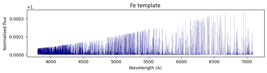
The atmospheric template must have a wavelength vector in the same units as the data and the flux must be normalised (around 1.0). For this example we use the Fe template (download here) generated with petitRADTRANS.
[9]:
template_path = data_dir + 'Fe_tea_template.npy'
twave, tflux = np.load(template_path)

template = Template(wlt=twave, flux=tflux).sort()

fig, ax = plt.subplots(1, figsize=(10,2))
ax.plot(template.wlt, template.flux, c='navy', lw=0.1)
ax.set(xlabel='Wavelength (A)', ylabel='Normalised flux', title='Fe template')
plt.show()
Compute the CCF
Pass an RV-lag vector to compute the CCF at each RV, thus generating a CCF-map. The step-size of the RV should be greater (or equal) to the instrumental resolution. For HARPS-N: R ~ 115,000 —> \(\Delta\)v ~ 1 km/s.
[10]:
dRV = 1.
RVt = np.arange(-350,350+dRV, dRV)

# Define CCF object
ccf = CCF(rv=RVt, template=template)
ccf.run(dcm, noise='var')
CCF elapsed time: 2.74 s
[10]:
<redcross.cross_correlation.CCF at 0x7fa8655b7dc0>
Load planet data
To shift the CCF to the planetary rest-frame we need to load the planet’s orbital parameters.
from a file
[11]:
planet_file = 'data/wasp189.dat'
planet = Planet(file=planet_file)
manually passing a dictionary
[15]:
planet_dict = {'P':2.7240338, 'a':0.0497, 'i':84.32, 'v_sys':-20.82, 'Tc_jd':2456706.4558, 'T_14':4.351199999,
               'RA_DEG': 225.68695,'DEC_DEG': -3.0313833}
planet = Planet(**planet_dict)
planet.BERV = header.BERV
planet.MJD = header.MJD
Shift the CCF to the planetary rest frame (PRF)
Each frame is shifted by the expected radial velocity of the planet at each time (at mid-exposure).
[16]:
fig, ax = plt.subplots(3,1,figsize=(6,10))

ccf.imshow(ax=ax[0])
ccf_planet = ccf.to_planet_frame(planet, ax=ax[1])
ax[2].plot(ccf_planet.rv, np.median(ccf_planet.flux, axis=0))

ax[0].set(ylabel='Frame number', title='CCF-map in stellar RF')
ax[1].set(ylabel='Frame number', title='CCF-map in planetary RF')
ax[2].set(xlabel='RV (km/s)', ylabel='CCF value', title='CCF average over time (planetary RF)')
plt.show()

Kp-Vsys map
This map is constructed by adding the values of the CCF along different paths by changing the \(K_p\) and \(V_{sys}\) values. The planet signal should appear around $V_{sys} \sim `$ 0 km/s if the passed :math:`V_{sys} value is correct. The \(K_p\) vector is automatically generated around the expected \(K_p\) (with the planet orbital parameters):
The instantaneous planet velocity is (in the observer’s and planet’s reference frame):
where \(\phi\) is the phase (\(\phi = 0\) at mid-transit planet.Tc).
[17]:
kpv = KpV(ccf, planet)
kpv.run() # compute the kpv-map values
kpv.fancy_figure() # display the map with 1D-plots
plt.show()
print('Expected planet Kp = {:.1f} km/s'.format(planet.Kp))
Horizontal slice at Kp = 197.5 km/s
Vertical slice at Vrest = 2.0 km/s

Expected planet Kp = 197.5 km/s